论文答辩PPT里面的数据
之前有jupyter notebook写的这些图,然后打算记录一下,就直接导出了md形式。
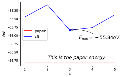
c6的能量情况
import matplotlib.pyplot as plt
import numpy as np
plt.figure()

x = [1,2,3,4,5]

c6 = [-55.449811,-55.087660,-55.842908,-55.769555,-55.392726]  #c6
c4 = [-55.194036,-55.431466,-55.352108,-54.958140,-55.324936]
y = [-56.8225,-56.8225,-56.8225,-56.8225,-56.8225]

plt.xlabel('x')
plt.ylabel('y/$eV$')
plt.text(2,-56.70,r'$This\ is\ the\ paper\ energy.$',fontdict={'size':16,'color':'k'})

new_ticks = [1,2,3,4,5]
print(new_ticks)
plt.xticks(new_ticks)
plt.plot(x,y,label='paper',color='r')

# 对c6进行标记
plt.plot(x,c6,label='c6',color='b')
c6x = 3
c6y = -55.842908
plt.scatter(c6x,c6y,s=50,color='b')
plt.annotate('$E_{min}=-55.84eV$',xy=(c6x,c6y),xycoords='data',xytext=(+30,-30),textcoords='offset points',fontsize=16,arrowprops=dict(arrowstyle='->',connectionstyle='arc3,rad=.2'))

plt.legend(loc='best',prop={'size': 13})
[1, 2, 3, 4, 5]


<matplotlib.legend.Legend at 0x1acec5c1d30>
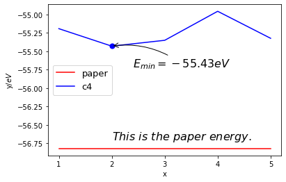
C4能量情况
import matplotlib.pyplot as plt
import numpy as np
plt.figure()

x = [1,2,3,4,5]

y = [-56.8225,-56.8225,-56.8225,-56.8225,-56.8225]
c4 = [-55.194036,-55.431466,-55.352108,-54.958140,-55.324936]

plt.xlabel('x')
plt.ylabel('y/$eV$')
plt.text(2,-56.70,r'$This\ is\ the\ paper\ energy.$',fontdict={'size':16,'color':'k'})

new_ticks = [1,2,3,4,5]
print(new_ticks)
plt.xticks(new_ticks)
plt.plot(x,y,label='paper',color='r')

# 对c4进行标记
plt.plot(x,c4,label='c4',color='b')
c6x = 2
c6y = -55.43
plt.scatter(c6x,c6y,s=50,color='b')
plt.annotate('$E_{min}=%s eV$'%c6y ,xy=(c6x,c6y),xycoords='data',xytext=(+30,-30),textcoords='offset points',fontsize=16,arrowprops=dict(arrowstyle='->',connectionstyle='arc3,rad=.2'))

plt.legend(loc=6,prop={'size': 13})
[1, 2, 3, 4, 5]


<matplotlib.legend.Legend at 0x1acec4e04c0>
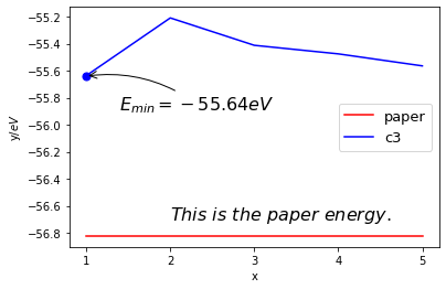
c3能量情况
import matplotlib.pyplot as plt
import numpy as np
plt.figure()

x = [1,2,3,4,5]

y = [-56.8225,-56.8225,-56.8225,-56.8225,-56.8225]
c3 = [-55.636299,-55.209602,-55.412220,-55.475558,-55.564359]

plt.xlabel('x')
plt.ylabel('y/$eV$')
plt.text(2,-56.70,r'$This\ is\ the\ paper\ energy.$',fontdict={'size':16,'color':'k'})

new_ticks = [1,2,3,4,5]
print(new_ticks)
plt.xticks(new_ticks)
plt.plot(x,y,label='paper',color='r')

# 对c3进行标记
plt.plot(x,c3,label='c3',color='b')
c3x = 1
c3y = -55.64
plt.scatter(c3x,c3y,s=50,color='b')
plt.annotate('$E_{min}=%s eV$'%c3y ,xy=(c3x,c3y),xycoords='data',xytext=(+30,-30),textcoords='offset points',fontsize=16,arrowprops=dict(arrowstyle='->',connectionstyle='arc3,rad=.2'))

plt.legend(loc='best',prop={'size': 13})
[1, 2, 3, 4, 5]


<matplotlib.legend.Legend at 0x1acec408ee0>
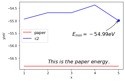
C2的能量情况
import matplotlib.pyplot as plt
import numpy as np
plt.figure()

x = [1,2,3,4,5]

y = [-56.8225,-56.8225,-56.8225,-56.8225,-56.8225]
c2 = [-54.937669,-54.682954,-54.686049,-54.375611,-54.994643]

plt.xlabel('x')
plt.ylabel('y/$eV$')
plt.text(2,-56.70,r'$This\ is\ the\ paper\ energy.$',fontdict={'size':16,'color':'k'})

new_ticks = [1,2,3,4,5]
print(new_ticks)
plt.xticks(new_ticks)
plt.plot(x,y,label='paper',color='r')

# 对c2进行标记
plt.plot(x,c2,label='c2',color='b')
c2x = 5
c2y = -54.99
plt.scatter(c2x,c2y,s=50,color='b')
plt.annotate('$E_{min}=%s eV$'%c2y ,xy=(c2x,c2y),xycoords='data',xytext=(-150,-50),textcoords='offset points',fontsize=16,arrowprops=dict(arrowstyle='->',connectionstyle='arc3,rad=.2'))

plt.legend(loc=6,prop={'size': 13})
[1, 2, 3, 4, 5]


<matplotlib.legend.Legend at 0x1acec39d220>
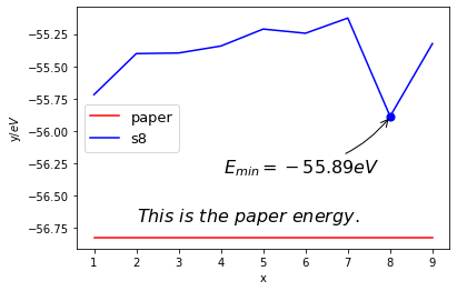
8份
import matplotlib.pyplot as plt
import numpy as np
plt.figure()

x = [1,2,3,4,5,6,7,8,9]

y = [-56.8225,-56.8225,-56.8225,-56.8225,-56.8225,-56.8225,-56.8225,-56.8225,-56.8225]
s8 = [-55.719069,-55.402108,-55.397541,-55.343724,-55.212809,-55.245086,-55.127715,-55.886796,-55.325181]

plt.xlabel('x')
plt.ylabel('y/$eV$')
plt.text(2,-56.70,r'$This\ is\ the\ paper\ energy.$',fontdict={'size':16,'color':'k'})

new_ticks = [1,2,3,4,5,6,7,8,9]
print(new_ticks)
plt.xticks(new_ticks)
plt.plot(x,y,label='paper',color='r')

# 对8份进行标记
plt.plot(x,s8,label='s8',color='b')
s8x = 8
s8y = -55.89
plt.scatter(s8x,s8y,s=50,color='b')
plt.annotate('$E_{min}=%s eV$'%s8y ,xy=(s8x,s8y),xycoords='data',xytext=(-150,-50),textcoords='offset points',fontsize=16,arrowprops=dict(arrowstyle='->',connectionstyle='arc3,rad=.2'))

plt.legend(loc='best',prop={'size': 13})
[1, 2, 3, 4, 5, 6, 7, 8, 9]


<matplotlib.legend.Legend at 0x1acec0c8ee0>
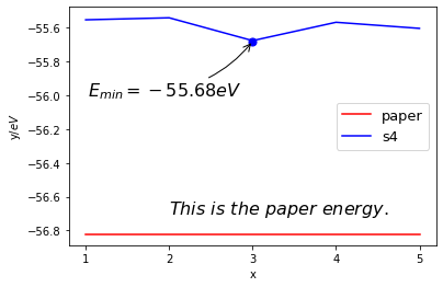
4份能量分布
import matplotlib.pyplot as plt
import numpy as np
plt.figure()

x = [1,2,3,4,5]

y = [-56.8225,-56.8225,-56.8225,-56.8225,-56.8225]
s4 = [-55.552306,-55.540388,-55.675706,-55.566915,-55.603029]

plt.xlabel('x')
plt.ylabel('y/$eV$')
plt.text(2,-56.70,r'$This\ is\ the\ paper\ energy.$',fontdict={'size':16,'color':'k'})

new_ticks = [1,2,3,4,5]
print(new_ticks)
plt.xticks(new_ticks)
plt.plot(x,y,label='paper',color='r')

# 对c4进行标记
plt.plot(x,s4,label='s4',color='b')
s4x = 3
s4y = -55.68
plt.scatter(s4x,s4y,s=50,color='b')
plt.annotate('$E_{min}=%s eV$'%s4y ,xy=(s4x,s4y),xycoords='data',xytext=(-150,-50),textcoords='offset points',fontsize=16,arrowprops=dict(arrowstyle='->',connectionstyle='arc3,rad=.2'))

plt.legend(loc='best',prop={'size': 13})
[1, 2, 3, 4, 5]


<matplotlib.legend.Legend at 0x1ace6892a00>
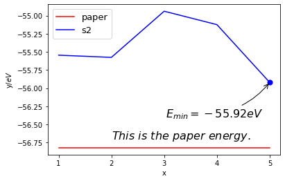
2份
import matplotlib.pyplot as plt
import numpy as np
plt.figure()

x = [1,2,3,4,5]

y = [-56.8225,-56.8225,-56.8225,-56.8225,-56.8225]
s2 = [-55.545215,-55.575504,-54.938865,-55.123865,-55.920604]

plt.xlabel('x')
plt.ylabel('y/$eV$')
plt.text(2,-56.70,r'$This\ is\ the\ paper\ energy.$',fontdict={'size':16,'color':'k'})

new_ticks = [1,2,3,4,5]
print(new_ticks)
plt.xticks(new_ticks)
plt.plot(x,y,label='paper',color='r')

# 对c4进行标记
plt.plot(x,s2,label='s2',color='b')
s2x = 5
s2y = -55.92
plt.scatter(s2x,s2y,s=50,color='b')
plt.annotate('$E_{min}=%s eV$'%s2y ,xy=(s2x,s2y),xycoords='data',xytext=(-150,-50),textcoords='offset points',fontsize=16,arrowprops=dict(arrowstyle='->',connectionstyle='arc3,rad=.2'))

plt.legend(loc='best',prop={'size': 13})
[1, 2, 3, 4, 5]


<matplotlib.legend.Legend at 0x1acea976fd0>
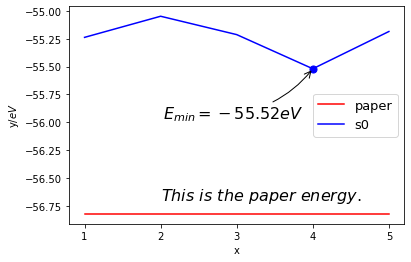
不分割
import matplotlib.pyplot as plt
import numpy as np
plt.figure()

x = [1,2,3,4,5]

y = [-56.8225,-56.8225,-56.8225,-56.8225,-56.8225]
s0 = [-55.237822,-55.048236,-55.213191,-55.519570,-55.185109]

plt.xlabel('x')
plt.ylabel('y/$eV$')
plt.text(2,-56.70,r'$This\ is\ the\ paper\ energy.$',fontdict={'size':16,'color':'k'})

new_ticks = [1,2,3,4,5]
print(new_ticks)
plt.xticks(new_ticks)
plt.plot(x,y,label='paper',color='r')

# 对c4进行标记
plt.plot(x,s0,label='s0',color='b')
s0x = 4
s0y = -55.52
plt.scatter(s0x,s0y,s=50,color='b')
plt.annotate('$E_{min}=%s eV$'%s0y ,xy=(s0x,s0y),xycoords='data',xytext=(-150,-50),textcoords='offset points',fontsize=16,arrowprops=dict(arrowstyle='->',connectionstyle='arc3,rad=.2'))

plt.legend(loc='best',prop={'size': 13})
[1, 2, 3, 4, 5]


<matplotlib.legend.Legend at 0x1ace924d4f0>
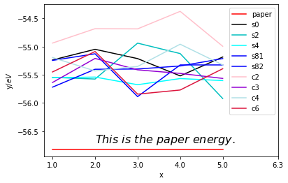
将所有的线放在一起
import matplotlib.pyplot as plt
import numpy as np
plt.figure()

x = [1,2,3,4,5]

y = [-56.8225,-56.8225,-56.8225,-56.8225,-56.8225]

s0 = [-55.237822,-55.048236,-55.213191,-55.519570,-55.185109]
s2 = [-55.545215,-55.575504,-54.938865,-55.123865,-55.920604]
s4 = [-55.552306,-55.540388,-55.675706,-55.566915,-55.603029]
s81 = [-55.719069,-55.402108,-55.397541,-55.343724,-55.212809]
s82 = [-55.245086,-55.127715,-55.886796,-55.325181,-55.325181]
c2 = [-54.937669,-54.682954,-54.686049,-54.375611,-54.994643]
c3 = [-55.636299,-55.209602,-55.412220,-55.475558,-55.564359]
c6 = [-55.449811,-55.087660,-55.842908,-55.769555,-55.392726]  #c6
c4 = [-55.194036,-55.431466,-55.352108,-54.958140,-55.324936]


plt.plot(x,y,label='paper',color='r')

# 对s0进行标记
plt.plot(x,s0,label='s0',color='k')

# 对2份进行标记
plt.plot(x,s2,label='s2',color='c')

# 对4进行标记
plt.plot(x,s4,label='s4',color='aqua')

# 对8份进行标记
plt.plot(x,s81,label='s81',color='b')
plt.plot(x,s82,label='s82',color='b')

# 对c2进行标记
plt.plot(x,c2,label='c2',color='pink')

# 对c3进行标记
plt.plot(x,c3,label='c3',color='darkviolet')

# 对c4进行标记
plt.plot(x,c4,label='c4',color='powderblue')

# 对c6进行标记
plt.plot(x,c6,label='c6',color='crimson')

plt.xlabel('x')
plt.ylabel('y/$eV$')
plt.text(2,-56.70,r'$This\ is\ the\ paper\ energy.$',fontdict={'size':16,'color':'k'})

new_ticks = [1,2,3,4,5,6.3]
print(new_ticks)
plt.xticks(new_ticks)

plt.legend(loc=1,prop={'size': 10})
plt.show()
[1, 2, 3, 4, 5, 6.3]
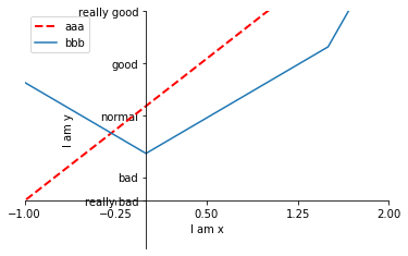
the example
画图的一些基本操作:
包括,横纵坐标轴的label,ticks,linewidth,color,linestyle,legend,handles,labels等等
更改坐标原点gca,spines,xaxis,yaxis
import matplotlib.pyplot as plt
import numpy as np

x = np.linspace(-3,3,5)
y1 = 2*x + 1
y2 = x**2

plt.figure(num=1)


plt.xlabel('I am x')
plt.ylabel('I am y')
plt.xlim((-1,2))
plt.ylim((-2,3))

new_ticks = np.linspace(-1,2,5)
#print(new_ticks)
plt.xticks(new_ticks)

plt.yticks([-1,-0.5,0.8,1.9,3],[r'really bad',r'bad',r'normal',r'good',r'really good'])


# gca = get current axis

ax = plt.gca()
ax.spines['right'].set_color('none')
ax.spines['top'].set_color('none')

ax.xaxis.set_ticks_position('bottom')    #改变原点位置
ax.yaxis.set_ticks_position('left')

ax.spines['bottom'].set_position(('data',-1))
ax.spines['left'].set_position(('data',0))


l1, = plt.plot(x,y1,color='red',linestyle='--',linewidth=2.0,label='up')
l2, = plt.plot(x,y2,label='down')

plt.legend(handles=[l1,l2,],labels=['aaa','bbb'],loc='best')    #
<matplotlib.legend.Legend at 0x1ace66478e0>
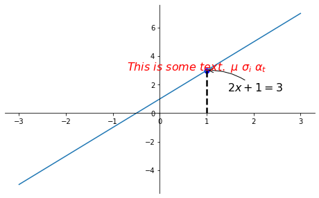
续
对图进行一些标记注解
# 画出基本图
import matplotlib.pyplot as plt
import numpy as np

x = np.linspace(-3, 3, 50)
y = 2*x + 1

plt.figure(num=1, figsize=(8, 5),)
plt.plot(x, y,)

# 移动坐标轴
ax = plt.gca()
ax.spines['right'].set_color('none')
ax.spines['top'].set_color('none')
ax.xaxis.set_ticks_position('bottom')
ax.spines['bottom'].set_position(('data', 0))
ax.yaxis.set_ticks_position('left')
ax.spines['left'].set_position(('data', 0))


x0 = 1
y0 = 2*x0 + 1
#plt.scatter()  散点图
plt.scatter(x0,y0,s=50,color='b')
plt.plot([x0,x0],[y0,0],'k--',lw=2.5) # 绘制一条竖直线  K 代表black

#method 1

plt.annotate(r'$2x+1=%s$' %y0,xy=(x0,y0),xycoords='data',xytext=(+30,-30),textcoords='offset points',fontsize=16,arrowprops=dict(arrowstyle='->',connectionstyle='arc3,rad=.2'))

plt.text(-.7,3,r'$This\ is\ some\ text.\ \mu\ \sigma_i\ \alpha_t$',fontdict={'size':16,'color':'r'})
plt.show()